Introduction

We work through a problem posed in Chapter 8 of [1].

from fastai.collab import *
from fastai.tabular.all import *
path = untar_data(URLs.ML_100k)

100.15% [4931584/4924029 00:00<00:00]

Path.BASE_PATH = path
path.ls()

(#23) [Path('u1.base'),Path('u1.test'),Path('u4.test'),Path('allbut.pl'),Path('u.item'),Path('ua.test'),Path('u.occupation'),Path('u3.test'),Path('u5.base'),Path('ub.test')...]

ratings = pd.read_csv(path/'u.data', delimiter='\t', header=None,
                     names=['user','movie','rating','timestamp'])
ratings.head()

	user	movie	rating	timestamp
0	196	242	3	881250949
1	186	302	3	891717742
2	22	377	1	878887116
3	244	51	2	880606923
4	166	346	1	886397596

We see that the rating can be one of the following values:

ratings.rating.unique()

array([3, 1, 2, 4, 5])

movies = pd.read_csv(path/'u.item', delimiter='|', encoding='latin-1',
                     usecols=(0,1), names=('movie','title'), header=None)
movies.head()

	movie	title
0	1	Toy Story (1995)
1	2	GoldenEye (1995)
2	3	Four Rooms (1995)
3	4	Get Shorty (1995)
4	5	Copycat (1995)

ratings = ratings.merge(movies)
ratings.head()

	user	movie	rating	timestamp	title
0	196	242	3	881250949	Kolya (1996)
1	63	242	3	875747190	Kolya (1996)
2	226	242	5	883888671	Kolya (1996)
3	154	242	3	879138235	Kolya (1996)
4	306	242	5	876503793	Kolya (1996)

DataLoaders

dls = CollabDataLoaders.from_df(ratings, item_name='title', bs=64)
dls.show_batch()

	user	title	rating
0	328	Star Trek VI: The Undiscovered Country (1991)	3
1	251	Toy Story (1995)	4
2	456	Judgment Night (1993)	2
3	653	Raiders of the Lost Ark (1981)	5
4	551	Aliens (1986)	4
5	416	Edge, The (1997)	4
6	116	Good Will Hunting (1997)	3
7	500	Chain Reaction (1996)	3
8	393	Barb Wire (1996)	3
9	227	Father of the Bride Part II (1995)	3

Probabilistic Matrix Factorization baseline

Underneath the covers we have a dot product model (where the dot product is between the user embedding and the item embedding). We use L2 regularization (wd=0.5) and use y_range to make sure the sigmoid_range can get to a rating of \(5\). Recall that in the sigmoid function only an activation of \(\infty\) will get us a \(1\). This will use the MSE as the loss function.

learn = collab_learner(dls, n_factors=50, y_range=(0,5.5))
learn.fit_one_cycle(5, 5e-3, wd=0.1)

epoch	train_loss	valid_loss	time
0	0.938077	0.954516	00:09
1	0.845044	0.872871	00:09
2	0.723613	0.843354	00:18
3	0.586253	0.829404	00:09
4	0.491200	0.829491	00:10

So \(0.829\) is what we want to beat!

Deep Learning baseline

Instead of a Dot Product model we use a model where the user and the movie embeddings are concatenated together and then passed through a neural net. We continue to use MSE as our loss.

learn2 = collab_learner(dls, n_factors=50, use_nn=True, layers=[100], y_range=(0,5.5))
learn2.fit_one_cycle(5, 5e-3, wd=0.1)

epoch	train_loss	valid_loss	time
0	0.991514	0.999929	00:12
1	0.940058	0.930773	00:13
2	0.867342	0.879026	00:12
3	0.810829	0.855366	00:12
4	0.753963	0.852470	00:12

The model is as follows:

learn2.model

EmbeddingNN(
  (embeds): ModuleList(
    (0): Embedding(944, 74)
    (1): Embedding(1665, 102)
  )
  (emb_drop): Dropout(p=0.0, inplace=False)
  (bn_cont): BatchNorm1d(0, eps=1e-05, momentum=0.1, affine=True, track_running_stats=True)
  (layers): Sequential(
    (0): LinBnDrop(
      (0): Linear(in_features=176, out_features=100, bias=False)
      (1): ReLU(inplace=True)
      (2): BatchNorm1d(100, eps=1e-05, momentum=0.1, affine=True, track_running_stats=True)
    )
    (1): LinBnDrop(
      (0): Linear(in_features=100, out_features=1, bias=True)
    )
    (2): SigmoidRange(low=0, high=5.5)
  )
)

Cross Entropy Loss

Turn each rating into a class label by subtracting one. Recall we saw that ratings are integers from \(1\) to \(5\).

ratings['class'] = ratings['rating'] - 1
ratings.head(n=5)

	user	movie	rating	timestamp	title	class
0	196	242	3	881250949	Kolya (1996)	2
1	63	242	3	875747190	Kolya (1996)	2
2	226	242	5	883888671	Kolya (1996)	4
3	154	242	3	879138235	Kolya (1996)	2
4	306	242	5	876503793	Kolya (1996)	4

ratings['class'].unique()

array([2, 4, 3, 1, 0])

dls3 = CollabDataLoaders.from_df(ratings, item_name='title', rating_name='class', bs=64)
dls3.show_batch()

	user	title	class
0	581	Return of the Jedi (1983)	2
1	159	Courage Under Fire (1996)	3
2	521	Long Kiss Goodnight, The (1996)	3
3	533	Stupids, The (1996)	0
4	77	Brazil (1985)	3
5	12	Lion King, The (1994)	3
6	605	Usual Suspects, The (1995)	3
7	561	Richard III (1995)	2
8	246	Doors, The (1991)	0
9	658	Boot, Das (1981)	4

Create a class that is able to output as many activations as there are classes.

class CollabNN(Module):
    def __init__(self, user_sz, item_sz, n_act=100, n_classes=5):
        self.user_factors = Embedding(*user_sz)
        self.item_factors = Embedding(*item_sz)
        self.layers = nn.Sequential(
            nn.Linear(user_sz[1]+item_sz[1], n_act),
            nn.ReLU(),
            nn.Linear(n_act, n_classes))
        
    def forward(self, x):
        embs = self.user_factors(x[:,0]),self.item_factors(x[:,1])
        return self.layers(torch.cat(embs, dim=1))

embs = get_emb_sz(dls3)
embs

[(944, 74), (1665, 102)]

model = CollabNN(*embs)

Examine a batch of inputs and outputs

x, y = dls3.one_batch()
x[:3], y[:3]

(tensor([[ 763, 1211],
         [ 474, 1006],
         [ 261,  734]]), tensor([[3],
         [4],
         [3]], dtype=torch.int8))

Get activations by passing through the model

model(x[:3])

tensor([[ 0.1065, -0.0083, -0.1098, -0.1151, -0.0471],
        [ 0.1053, -0.0053, -0.1108, -0.1145, -0.0490],
        [ 0.1017, -0.0110, -0.1114, -0.1135, -0.0478]],
       grad_fn=<AddmmBackward0>)

Apply softmax to the activations

torch.softmax(model(x[:3]), dim=-1)

tensor([[0.2296, 0.2047, 0.1849, 0.1839, 0.1969],
        [0.2293, 0.2053, 0.1848, 0.1841, 0.1965],
        [0.2289, 0.2045, 0.1850, 0.1846, 0.1971]], grad_fn=<SoftmaxBackward0>)

Take the argmax to get the prediction of the class

torch.softmax(model(x[:3]), dim=-1).argmax(dim=-1)

tensor([0, 0, 0])

Unsqueeze to match the shape of the y’s

torch.softmax(model(x[:3]), dim=-1).argmax(dim=-1).unsqueeze(-1)

tensor([[0],
        [0],
        [0]])

Convert to float and compute the mse_loss

F.mse_loss(torch.softmax(model(x[:3]), dim=-1).argmax(dim=-1).unsqueeze(-1).float(), y[:3])

tensor(11.3333)

Create our custom mse function that can get a loss from these activations for the different classes. We do this so we can compare the validation loss metric against the previous baselines. Clearly cross entropy loss cannot be compared directly to the mean squared error.

def ks_mse(inp, targ, axis=-1):
    sm_acts = torch.softmax(inp, dim=-1)
    preds = sm_acts.argmax(dim=axis).unsqueeze(-1)
    return F.mse_loss(preds.float(), targ)

Compare with our custom function

ks_mse(model(x[:3]), y[:3])

tensor(11.3333)

learn3 = Learner(dls3, model, loss_func=CrossEntropyLossFlat(), metrics=[accuracy, ks_mse])

lrs = learn3.lr_find()

lrs

SuggestedLRs(valley=0.0012022644514217973)

learn3.fit_one_cycle(5, lrs.valley)

epoch	train_loss	valid_loss	accuracy	ks_mse	time
0	1.177951	1.238908	0.444100	1.217100	00:13
1	1.186859	1.232669	0.448450	1.215550	00:13
2	1.168161	1.228795	0.452750	1.146900	00:12
3	1.132046	1.233022	0.451050	1.154100	00:12
4	1.096163	1.237107	0.450800	1.162600	00:13

Unfortunately, in this attempt, we came up short and were unable to beat the baseline.

Finally, let’s use a confusion matrix to visualize where this model is coming up short.

raw_preds, targs, decoded_preds = learn3.get_preds(with_decoded=True)
raw_preds[:3], decoded_preds[:3], targs[:3]

(tensor([[0.0255, 0.2153, 0.2651, 0.4588, 0.0353],
         [0.0089, 0.0586, 0.2399, 0.4129, 0.2797],
         [0.0028, 0.1422, 0.3484, 0.3990, 0.1076]]),
 tensor([3, 3, 3]),
 tensor([[4],
         [4],
         [3]], dtype=torch.int8))

from sklearn.metrics import ConfusionMatrixDisplay
ConfusionMatrixDisplay.from_predictions(targs, decoded_preds)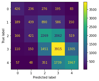

<sklearn.metrics._plot.confusion_matrix.ConfusionMatrixDisplay>

from sklearn.metrics import classification_report
print(classification_report(targs, decoded_preds, labels=[0, 1, 2, 3, 4]))

              precision    recall  f1-score   support

           0       0.45      0.35      0.39      1216
           1       0.34      0.19      0.25      2254
           2       0.43      0.42      0.43      5437
           3       0.46      0.56      0.51      6931
           4       0.49      0.47      0.48      4162

    accuracy                           0.45     20000
   macro avg       0.43      0.40      0.41     20000
weighted avg       0.44      0.45      0.44     20000

References

[1]

J. Howard and S. Gugger, Deep learning for coders with fastai and PyTorch: AI applications without a PhD, 1st ed. O’Reilly, 2020.